Category: Technology

Programming, gadgets (reviews thereof) and computers

Gear review: Boss RC-3 Loop station

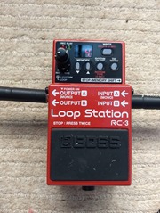
boss-loop-station-rc3In a change from usual service I am reviewing some guitar related gear: a Boss RC-3 Loop Station. Review is probably not the right word, this is the only guitar pedal of this type I’ve used so really this is more about describing what it does, which would be useful for other novices, capturing some of the instructions in a more readable form and sharing some resources.

A loop pedal is a device which records sound – pedals are devices designed to be activated with a foot. The intention of a loop pedal is to capture short sequences of sound which you then play over as they repeat in the background, so that one musician can make the sound of many. Ed Sheeran and KT Tunstall are particularly well-known users of the loop pedal, needless to say that despite owning one I sound no where near as good!

It’s worth noting that although this is advertised as a guitar pedal it will record any sound fed into the input side, I’ve used it with my electric drum kit, it will work with the keyboards we have and if I had a microphone I could sing into it (but nobody wants that).

There are plenty of loop pedals around, following a series of price points / sizes.The cheapest one in the Boss range is the RC-1 for something like £80, I paid £125 for the RC-3 which is one step up from the most basic models. Above the RC-3 in the Boss range are the RC-30 for £171 which has two large size foot switches and the RC-300 for £440 which is much larger and has footswitches for each of three tracks.

The RC-3 has 99 slots to record loops to, and will provide a rhythm track as well in one of 9 styles. There is a USB port which presents the pedal as a file directory, this allows you to backup your loops and save WAV files from elsewhere to it. I picked the Boss because I have a couple of other Boss devices (my amplifier and expression pedal) and I like the brand.

The device itself is nice and chunky, made out of metal. I think I prefer the big rubberised pedal style to the round metal push buttons found on other loop pedals. I found the other controls a bit small and fiddly, I’m not as young as I used to be – bending down and looking at small things are hard! Fundamentally this is a “small format device” problem which isn’t limited to the Boss pedal, space is limited to control the functionality provided so you get a two character display and five push buttons.

The buttons select the memory slot to be used (or cycle through options), select the rhythm functionality, write a loop to a memory slot and allow you to set the tempo of the rhythm track.

A couple of handy hints I picked up from this video by Reidy’s – a fine Lancashire company: firstly the default mode is that pedal presses take you from record to overdub to playback modes, you can change this to record to playback to overdub by holding down the tempo button whilst switching the device on. As a beginner this feels more natural. Secondly, you can clear, undo and redo the current loop by long presses on the pedal – so you can muck around recording and deleting little phrases with just the foot control. These features are both explained in the paper manual which comes with the device.

You can also change the record mode from the default, of starting recording as soon as the pedal is pressed, to auto recording which starts when you start playing and count-in which sounds the rhythm for a measure before recording starts.

The built-in rhythms are as follows:

  1. Hi-hat
  2. Kick & Hi-hat
  3. Rock 1
  4. Rock 2
  5. Pop
  6. Funk
  7. Shuffle
  8. R&B
  9. Latin
  10. Percussion

The tempo is set by tapping the tempo button, you can’t fix it to a specific value using the up and down buttons – most likely because the display can only handle a two digit tempo – and that’s a bit small.

One thing worth noting is if you have a Boss Katana 50 and an expression pedal you will not hear the effect of the expression pedal on the loop pedal recording. This is because the loop pedal is not seeing the expression pedal in its input. You can sort of capture it by putting the loop pedal on the output side of the Katana and plugging headphones, or another amplifier, into the loop pedal but it is not an ideal solution. Higher specification Boss Katana have an external effects loop which is where you would put the loop pedal. More generally the effects you hear on playback are the ones set on the amplifier at playback time, not those being used at record time.

Applications

I’ve already used the Boss for the following:

  • Fiddling about with amplifier tone – record a loop then adjust amplifier settings as it plays back – you don’t have to wrangle your guitar and amplifier at the same time and can hear immediately the effect of your knob twiddling;
  • Record your practicing – I use Yousician which has a lot of exercises – chords changes, fingerpicking, scales and the like. The loop pedal is an easy way to do a quick recording to hear where you are going wrong;
  • Simple rhythm track – it has a bunch of rhythm styles whose tempo you can adjust;
  • Backing chords to play over – I need to practice doing this;
  • Backing sounds from elsewhere

Summary

I am pleased with my purchase! I think it will take me quite a while to get to grips with recording a backing loop – I’ve been watching the Justin Guitar videos below to help me with this.

Resources

Scala – installation behind a workplace web proxy

I’ve been learning Scala as part of my continuing professional development. Scala is a functional language which runs primarily on the Java Runtime Environment. It is a first class citizen for working with Apache Spark – an important platform for data science. My intention in learning Scala is to get myself thinking in a more functional programming style and to gain easy access to Java-based libraries and ecosystems, typically I program in Python.

In this post I describe how to get Scala installed and functioning on a workplace laptop, along with its dependency manager, sbt. The core issue here is that my laptop at work puts me behind a web proxy so that sbt does not Just Work™. I figure this is a common problem so I thought I’d write my experience down for the benefit of others, including my future self.

The test system in this case was a relatively recent (circa 2015) Windows 7 laptop, I like using bash as my shell on Windows rather than the Windows Command Prompt – I install this using the Git for Windows SDK.

Scala can be installed from the Scala website https://www.scala-lang.org/download/. For our purposes we will use the  Windows binaries since the sbt build tool requires additional configuration to work. Scala needs the Java JDK version 1.8 to install and the JAVA_HOME needs to point to the appropriate place. On my laptop this is:

JAVA_HOME=C:\Program Files (x86)\Java\jdk1.8.0_131

The Java version can be established using the command:

javac –version

My Scala version is 2.12.2, obtained using:

scala -version

Sbt is the dependency manager and build tool for Scala, it is a separate install from:

http://www.scala-sbt.org/0.13/docs/Setup.html

It is possible the PATH environment variable will need to be updated manually to include the sbt executables (:/c/Program Files (x86)/sbt/bin).

I am a big fan of Visual Studio Code, so I installed the Scala helper for Visual Studio Code:

https://marketplace.visualstudio.com/items?itemName=dragos.scala-lsp

This requires a modification to the sbt config file which is described here:

http://ensime.org/build_tools/sbt/

Then we can write a trivial Scala program like:

object HelloWorld {


def main(args: Array[String]): Unit = {


    println(“Hello, world!”)


  }


}

And run it at the commandline with:

scala first.scala

To use sbt in my workplace requires proxies to be configured. The symptom of a failure to do this is that the sbt compile command fails to download the appropriate dependencies on first run, as defined in a build.sbt file, producing a line in the log like this:

[error] Server access Error: Connection reset url=https://repo1.maven.org/maven2/net/
sourceforge/htmlcleaner/htmlcleaner/2.4/htmlcleaner-2.4.pom

In my case I established the appropriate proxy configuration from the Google Chrome browser:

chrome://net-internals/#proxy

This shows a link to the pacfile, something like:

http://pac.madeupbit.com/proxy.pac?p=somecode

The PAC file can be inspected to identify the required proxy, in my this case there is a statement towards the end of the pacfile which contains the URL and port required for the proxy:

if (url.substring(0, 5) == ‘http:’ || url.substring(0, 6) == ‘https:’ || url.substring(0, 3) == ‘ws:’ || url.substring(0, 4) == ‘wss:’)

{

return ‘PROXY longproxyhosturl.com :80’;

}


These are added to a SBT_OPTS environment variable which can either be set in a bash-like .profile file or using the Windows environment variable setup.

export SBT_OPTS=”-Dhttps.proxyHost=longproxyhosturl.com -Dhttps.proxyPort=80 -Dhttps.proxySet=true”

As a bonus, if you want to use Java’s Maven dependency management tool you can use the same proxy settings but put them in a MAVEN_OPTS environment variable.

Typically to start a new project in Scala one uses the sbt new command with a pointer to a g8 template, in my workplace this does not work as normally stated because it uses the github protocol which is blocked by default (it runs on port 9418). The normal new command in sbt looks like:

sbt new scala/scala-seed.g8

The workaround for this is to specify the g8 repo in full including the https prefix:

sbt new https://github.com/scala/scala-seed.g8

This should initialise a new project, creating a whole bunch of standard directories.

So far I’ve completed one small project in Scala. Having worked mainly in dynamically typed languages it was nice that, once I had properly defined my types and got my program to compile, it ran without obvious error. I was a bit surprised to find no standard CSV reading / writing library as there is for Python. My Python has become a little more functional as a result of my Scala programming, I’m now a bit more likely to map a function over a list rather than loop over the list explicitly.

I’ve been developing intensively in Python over the last couple of years, and this seems to have helped me in configuring my Scala environment in terms of getting to grips with module/packaging, dependency managers, automated doocumentation building and also in finding my test library (http://www.scalatest.org/) at an early stage.

The Logging module in Python

In the spirit of improving my software engineering practices I have been trying to make more use of the Python logging module. In common with many programmers my first instinct when debugging a programming problem is to use print statements (or their local equivalent) to provide an insight into what my program is up to. Obviously, I should be making use of any debugger provided but there is something reassuring about the immediacy and simplicity of print.

A useful evolution of the print statement in Python is the logging module which can be used as a simple print function but it can do so much more: you can configure loggers for different packages and modules whose behaviour can be controlled centrally; you can vary the verbosity of your logging messages. If you decide to switch to logging to a file rather than the terminal this can be achieved too, and you can even post your log messages to a website using HTTPhandler. Obviously logging is about much more than debugging.

I am writing this blog post because, as most of us have discovered, using logging is not quite as straightforward as we were led to believe. In particular you might find yourself in the situation where you feel you have set up your logging yet when you run your code nothing appears in your terminal window. Print doesn’t do this to you!

Loggers are arranged in a hierarchy. Loggers have handlers which are the things that cause a log to generate output to a device. If no log is specified then a default log called the root log is used. A logger has a name and the hierarchy is defined by the dots in the name, all the way “up” to the root logger. Any logger can have a handler attached to it, if no handler is attached then any log message is passed to the parent logger.

A log record has a message (the thing you would have printed) and a “level” which indicates the severity of the message these are specified by integers for which the logging module provides convenient labels. The levels in order of severity are logging.DEBUG, logging.INFO, logging.WARNING, logging.ERROR, logging.CRITICAL. A log handler will output a message if the level of the message is equal to or more than the level it has been set to. So a handler set to WARNING will show messages at the WARNING, ERROR and CRITICAL levels but not the INFO and DEBUG levels.

The simplest way to use the logging module is to import the library:

import logging

Then carry out some minimal configuration,

logging.basicConfig(level=logging.INFO)

and then put logging.info statements in our code, just as we would have done with print statements:

logging.info("This is a log message that takes a parameter = {}".format(a_parameter_value))

logging.debug, logging.warning, logging.error and logging.critical are used to publish log messages with different levels of severity. These are all convenience methods which remove the need to explicitly give the level as found in the logging.log function:

logging.log(logging.INFO, "This is a log message")

If we are writing a module, or other code that we anticipate others importing and running then we should create a logger using logging.getLogger(__name__) but leave configuring it to the caller. In this instance we use the name of the logger we have created instead of the module level “logging”. So to publish a message we would do:

logger = logging.getLogger(__name__)
logger.info("Hello")

In the module importing this library you would do something like:

import some_library
logging.basicConfig(level=logging.INFO)
# if you wanted to tweak the levels of another logger 
logger = logging.getLogger("some other logger")
logger.setLevel(logging.DEBUG)

basicConfig() configures the root logger which is where all messages end up in the absence of any other handler. The behaviour of logging.basicConfig() is downright obstructive at times. The core of the problem is that it can only be invoked once in a session, any future invocations are ignored. Worse than this it can be invoked implicitly. So if for example you do:

import logging
logging.warning("Hello")

You’ll see a message because secretly logging has effectively run logging.basicConfig(level=logging.WARNING) for you (or something similar). This means that if you were to then naively go ahead and run basicConfig yourself:

logging.basicConfig(level=logging.INFO)

You would see no message when you subsequently ran logging.info(“Hello”) because the “second” invocation of logging.basicConfig is ignored.

We can explicitly set the properties of the root logger by doing:

root_logger = logging.getLogger()
root_logger.setLevel(logging.INFO)

You can debug issues like this by checking the handlers to a logger. If you do:

import logging
lgr = logging.getLogger()
lgr.handlers

You get the empty list []. Issue a logging.warning() message and you see that a handler has been added to the root logger, lgr.handlers() returns something like [<logging.StreamHandler at 0x44327f0>].

If you want to see a list of all the loggers in the hierarchy then do:

logging.Logger.manager.loggerDict

So there you go, the logging module is great – you should use it instead of print. But beware of the odd behaviour of logging.basicConfig() which I’ve spent most of this post griping about. This is mainly so that I have all my knowledge of logging in one place rather than trying to remember which piece of code I pulled off a particular trick.

I used the logging documentation here, blog posts by Fang (here) and Praveen Gollakota (here) and tab completion in the ipython REPL in the preparation of this post.

Parsing XML and HTML using xpath and lxml in Python

For the last few years my life has been full of the processing of HTML and XML using the lxml library for Python and the xpath query language. xpath is a query language designed specifically to search XML, unlike regular expressions which should definitely not be used to process XML related languages. Typically this has involved a lot of searching my own code to remind me how to do stuff. This blog post captures some handy snippets to avoid the inevitable Googling, and solidify for me exactly what I’ve been doing for the last few years!

But what does it {xml, html} look like?

xml and html are made up of “elements”, delimited by pointy brackets and attributes which are equal to things:

<element1 attribute1=”thing”>content</element1>

Elements can be nested inside other elements to make a tree structure. A wrinkle to be aware of is the so-called “tail” of an element. This is most often seen with <br/> tags (I think it is general):

<element1 attribute1=”thing”>content</br>tail</element1>

The “content” is accessed using text(), whilst the tail is accessed using .tail.

Web pages are made from HTML which is a “relaxed” XML format. XML is the basis of many other file formats found in the wild (such as GPX and GML). Dealing with XML is very similar to dealing with HTML except for namespaces, which I discuss in more detail at the end of this post.

XPath Helper

Before I get onto xpath I should introduce xpath helper – which is a plugin for Google Chrome which helps you develop xpath queries.

You can find XPath Helper in the Chrome Store, it is free. I use it in combination with the Google Chrome Developer tools, particular the “Inspect Element” functionality. XPath helper allows you to see the results of an xpath query live. You open up the XPath console (Ctrl+shift+x), type in your xpath and you see the results in both in the xpath helper console, and also as highlighting on the page.

You can get automatically generated xpath queries, however typically I have used these just as inspiration since they tend to be rather long and “brittle”.

Loading up the data

My Python scripts nearly always start with the following imports:

import lxml.html
import requests
import requests_cache
requests_cache.install_cache('demo_cache')

requests and requests_cache to access data on the web and lxml.html to parse the HTML. Then I can get a webpage using:

r = requests.get(url)
root = lxml.html.fromstring(r.content)

You might want to make any URLs absolute rather than relative:

root.make_links_absolute(base_url)

If I’m dealing with XML rather than HTML then I might do:

from lxml import etree

And then when it came to loading in a local XML file:

with open(input_file, "rb") as f:
	root = etree.XML(f.read())

XPath queries

With your root element in hand you can now get on with querying. Xpath queries are designed to extract a set of elements or attributes from an XML/HTML document by the name of the element, the value of an attribute on an element, by the relationship an element has with another element or by the content of an element.

Quite often xpath will return elements or lists of elements which, when printed in Python, don’t show you the content you want to see. To get the text content of an element you need to use .text, text_content(), or .tail, and make sure you ask for an array element rather than the whole array.

The follow examples show the key features of xpath. I’m using this blog (http:/www.ianhopkinson.org.uk/) as an example website so you can play along with xpath:

Specifying a complete path with / as separator

title = root.xpath('/html/body/div/div/div[2]/h1')

is the full path to my blog title. Notice how we request the 2nd element of the third set of div elements using div[2] – xpath arrays are one-based, not zero-based.

Specifying a path with wildcards using //

This expression also finds the title but the preamble of /html/body/div/div is absorbed by the // wildcard match:

title = root.xpath('//div[2]/h1')

To obtain the text of the title in Python, rather than an element object, we would do:

title_text = title[0].text.strip() or maybe title_text = title[0].text_content().strip()

text_content() would pick up any tail content, and any text in child elements. I use strip() here to remove leading and trailing whitespace

Selecting attribute values

we’ve seen that //element selects all of the elements of type “element”. We select attribute values like this:

ids = root.xpath('//li/@id')

which selects the id attribute from the list elements (li) on my blog

Specifying an element by attribute

We can select elements which have particular attribute values:

tagcloud = root.xpath('//*[@class="tagcloud"]')

this selects the tag cloud on my blog by selecting elements which having the class attribute “tagcloud”.

Select an element containing some specified text

We can do something similar with the text content of an element:

title = root.xpath(‘//h1[contains(., ‘SomeBeans’)]’)

This selects h1 elements which contain the text “SomeBeans”.

Select via a parent or sibling relationship

Sometimes we want to select elements by their relationship to another element, for example:

subtitle = root.xpath('//h1[contains(@class,"header_title")]/../h2')

this selects the h1 title of my blog (SomeBeans) then navigates to the parent with .. and selects the sibling h2 element (the subtitle “the makings of a small casserole”).

The same effect can be achieved with the following-sibling keyword:

subtitle = root.xpath('//h1[contains(@class,"header_title")]/following-sibling::h2')

XML Namespaces

When dealing with XML, we need to worry about namespaces. In principle the elements of an XML document are described in a schema which can be looked up and is universally unique. In practice the use of namespaces in XML documents can lead to much banging head against wall! This is largely because trivial examples of XML wrangling don’t use namespaces, except as a “special” example.

Here is a fragment of XML defining two namespaces:

<foo:Results xmlns:foo="http://www.foo.com" xmlns="http://www.bah.com">

xmlns:foo defines a namespace whose short form is “foo”, we select elements in this space using a namespace parameter to the xpath query:

records = root.xpath('//foo:Title', namespaces = {"foo": "http://www.foo.com"})

The “catch” here is we also define a default namespace xmlns = “http://www.bah.com”, which means that elements which don’t have a prefix cannot be selected unless we define the namespace in our xpath:

records = root.xpath('//bah:Title', namespaces = {"bah": http://www.bah.com})

Worse than that we need to include our namespace prefix in the query, even though it doesn’t appear in the file!

Conclusion

These snippets cover the majority of the xpath queries I’ve needed over the past few years, I’ll add any others as I find them. I’ve put all the code used here in a GitHub gist.

Xpath is the right tool for the job of extracting information from XML documents, including HTML – do not accept inferior alternatives!

Analysing LIDAR data for the UK

I’m currently between jobs for a couple of weeks, so I have time to play with data.

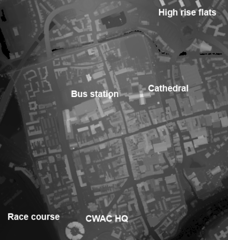
The Environment Agency (EA) has recently released it’s LIDAR data for England amounting to several terabytes of the stuff. LIDAR is a laser ranging technology which gives you the height profile of the surface under inspection. You can get a feel for the data from this excerpt of central Chester:

SJ46-Chester-512x512

The brightness of a pixel shows the height of a feature, so the race course (lower left) appears dark since it is a low flat region close to the River Dee. The CWAC HQ building is tall and appears bright. To the north of the city are a set of three high rise flats, which appear bright. The distinctive cross-shape of the cathedral, with it’s high, bright central tower is also visible. It’s immediately obvious that LIDAR is an excellent tool for picking out the footprint of buildings.

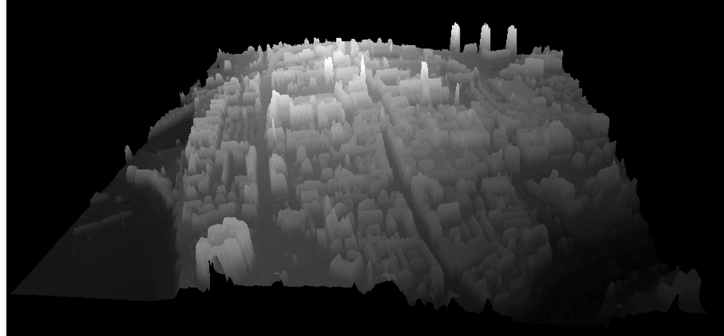
We can use the image above to make a 3D projection view where the brightness of a pixel is mapped to height:

Chester-3D

The orientation for this image is the same as that in the first image, the three tower blocks are visible top right, and the CWAC HQ visible lower left.

The images above used the lowest spatial resolution data, each pixel is 2mx2m. The data have released have spatial resolutions 2m down to 25cm for selected areas. Looking at the areas with the high resolution data available it becomes very obvious what the primary uses of the data are: flood and coastal defences.

You can find the LIDAR data here. It’s divided up into several datasets. Surface data gives height information including all objects on the land such as buildings, trees, vehicles and so forth whilst Terrain data is processed to remove these artefacts and show the pristine land surface.

Composite data are data compiled to give maximum coverage by combining data from surveys conducted in different years and at different resolutions whilst Tile data are the underlying raw data collected in different years and different resolutions. The coverage sliders show the coverage of each dataset. The data are for England only.

The images of Chester shown above are an excerpt from a 10kmx10km tile, shown below:

SJ46

Chester is on the left of this image, above the dark bend of River Dee flood plain. To the right hand side we can see the valley of the River Gowy, and its tributaries – features which are not obvious on the ground or in Google Maps. The large black area is where there is no data, smaller irregular black seem to correlate with water, you might just be able to pick out the line of the Shropshire Union canal cutting through the middle of the image.

I used Chester as an illustration because that’s where I live. I started looking at this data because I was curious, and I’ve spent a happy few days downloading data for lots of different places and playing with it.

It’s great to see data like this being released under permissive conditions. The Environment Agency has been collecting this data for its own purposes, and it’s been available from them commercially for a while – no doubt as a result of a central government edict to maximise revenue from it.

Opening the data like this means the curious can have a rummage, and perhaps others will find a commercial value in it.

I’ve included a few more images below. After them you can see the technical details of how to process these data and make the visualisations for yourself, the code is all in this GitHub repository:

https://github.com/IanHopkinson/defra-lidar-viewer

It is shared under the MIT license.

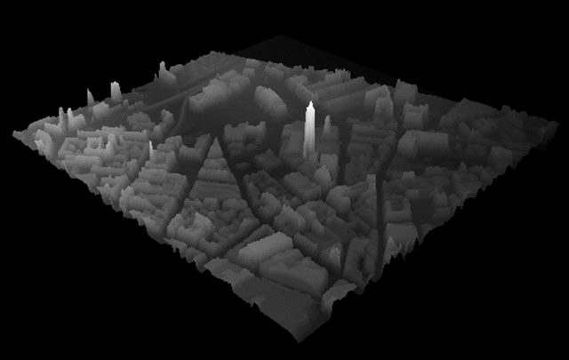
Liverpool in 3D with the Radio City tower

Liverpool-3D

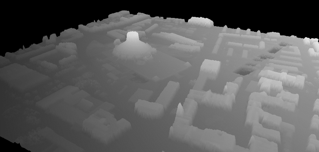
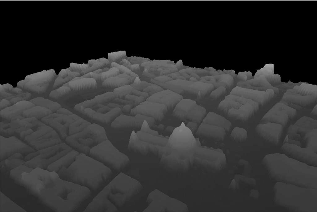
Liverpool Metropolitan Cathedral at 1m resolution

Liverpool-Metropolitan-cathedral-3D

St Paul’s Cathedral

StPauls-3D

Technical Details

The code used to make the figures in this blog post can be found here:

https://github.com/IanHopkinson/defra-lidar-viewer

The GitHub repository contains a readme file which describes the code, and provides links to the original data, other useful commentary and the numerous bits of code I borrowed from the internet.

The data start as sets of zipped text file archives, each archive contains the data for a 10kmx10km OS National Grid square – Chester is in the SJ46 cell. An archive contains a maximum of 100 text files, each one containing data for a single 1kmx1km square, the size of this file depends on the resolution of the data. I wrote a Python program to read the data for a 10kmx10km cell and convert it into a PNG format image. This program also calculates the bounding box in latitude and longitude for the cell. The processing program works fine for 2m and 1m resolution data. It works just about for 50cm data but is slow and throws memory errors. For 25cm resolution data it doesn’t yet work.

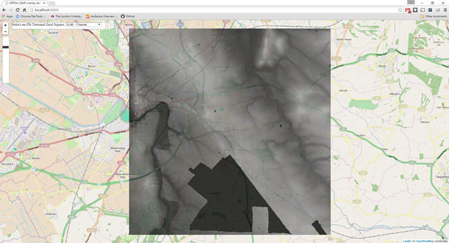
I made a visualisation using the leaflet.js library which allows you to overlay the PNG images generated above onto OpenStreetMap maps. The opacity of the image can be varied with a slider so that you can match LIDAR features to map features. The registration between the two data sources is pretty good but there are systematic problems which I believe might be due to different mapping projections being used by the Ordnance Survey and OpenStreetMap.

map-overlay

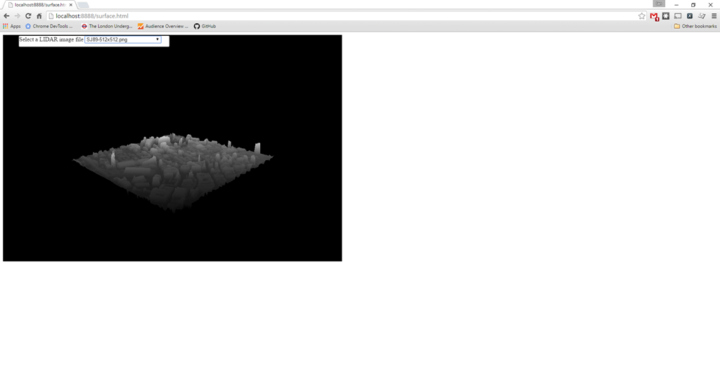
A second visualisation tool uses the three.js library to make an interactive 3D view. The input data are manual crops of approximately 512×512 from the raw PNGs, I did this using Paint .NET but other image editors would work fine. Larger images work but they are smoothed to 512×512 in the rendering. A gotcha here is that the revision number of the three.js library is important – the code for this visualisation leant heavily on previous work by others, and whilst integrating new functionality it was important to use three.js source files from the same revision. This visualisation allows you to manipulate the view with the mouse, it takes while to load up but once loaded it is pretty fast. Trying to upload a subsequent image doesn’t work.

3D-view

I’m still working on the code, I’d like to be able to process the 25cm data and it would be good to select an area from the map and convert it to 3D view automatically.